The Geometry Hidden in Data: An Introduction to Riemannian Metric Learning

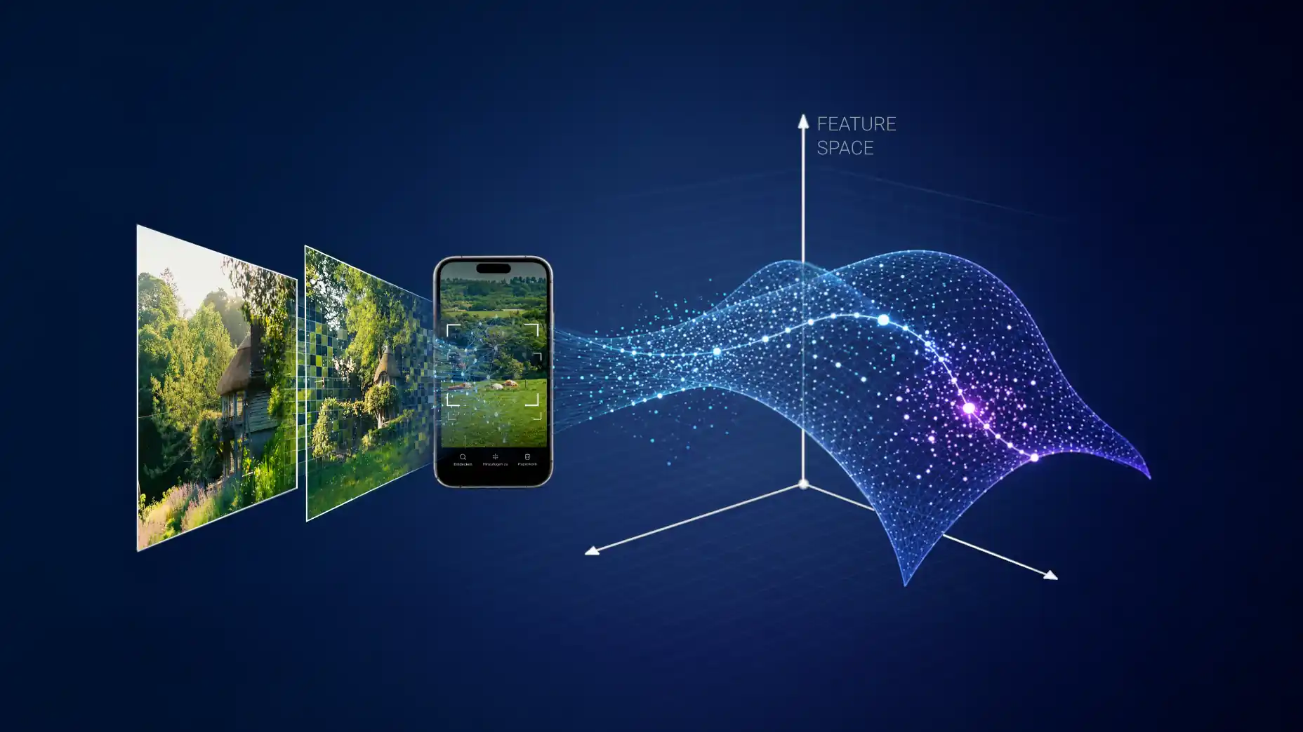
If you use any modern phone gallery app, one standout feature introduced in recent years is advanced face recognition. When you tap on a photo, the app can identify the people in it and lets you browse through all the pictures on your device where that person appears. It is especially remarkable in the sense that it recognizes faces across thousands of photos, even with varying lighting, angles, and expressions, and most astoundingly, through different ages.

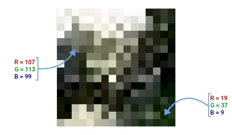
To elaborate on how remarkable this feat is, we’d have to understand how a computer, a non-thinking object, understands images. An image is a collection of pixels, which, when we are working with colour images, take three values representing the intensity of the colours red, green and blue (RGB). Each of these numbers between 0 (none of that colour) and 255 (as much as possible) specifies the contribution of each of the primary colours needed to produce a particular shade, similar to when we used to mix colours in kindergarten. An image is then a grid of such pixels.

Take a look at these pictures of a cottage taken on the same day, a side and a portrait view (cf. Fig. 2, left and middle panel). We as humans directly recognize that it is the same cottage. If we try to explain why we think that is, one might say that it has the same chimney, the roof is made of hay and is brown, even the trees surrounding its windows are the same. How would we explain that to a computer?

A good way of approximating “sameness” is by perceiving “closeness” or similarity. How different are two images from each other? This quantitative question is much more difficult to answer than its qualitative counterpart “Are these two images different?”

Mathematicians approach this issue by borrowing a concept from geometry: they introduce a notion of “distance” between images – or, more generally, between data sets. More precisely, they use a concept called a metric. In geometry, a metric is a mathematical function telling us how to calculate spatial distances between pairs of points.

To apply this idea to images (or any kind of data), we first describe them in the language of geometry. This is done by identifying measurable attributes in the image – so-called features. As discussed above, an image is essentially a grid of pixels, and each pixel is described by three numbers. We can therefore think of an image simply as a long list of numbers, one for each colour channel of each pixel. These numbers serve as coordinates. Taken together, they determine a single point in what mathematicians call feature space: an abstract space whose directions correspond to measurable properties of the data. In this case, each direction corresponds to one specific pixel colour value. A 62px × 62px image already gives rise to more than 11,500 such coordinates. Every image is thus represented as a point in this feature space. Two images that differ only slightly in their pixel values will be represented by nearby points. Images that differ strongly will lie far apart. The distance between two points in this space provides a quantitative notion of similarity.

Real images, of course, are characterized by far more than the colours of each pixel. A feature space can include any attributes of the data we deem important. For example, brightness, sharpness, edges, and textures are all relevant features of an image, and our perception of an image changes as these vary. Adding such features produces very high-dimensional feature spaces. Despite the large number of dimensions, the basic idea remains simple: each image occupies a precise position in feature space, and measuring distance between positions allows us to compare images.

Thus, geometry gives us a language for comparing data: distances encode similarity, different directions encode different measurable aspects of the image, and patterns formed by many points reflect structure within the data set.

In the geometry we learn at school, which is usually restricted to the study of flat surfaces and spaces, distance boils down to measuring the length of the straight line connecting two points, the way a ruler works in two dimensions. In that geometry, known as Euclidean geometry, there exists exactly one such line segment for each pair of points, as guaranteed by Euclid’s very first postulate (there are four more, we won’t get into that), and its length is easily found using the Pythagorean theorem (see the info box below). Since we also represent an image as a high-dimensional vector, we can apply the same formula in many dimensions and compute the distance between two images in this abstract feature space: the bigger the number, the further apart the images are deemed to be, and the less similar they should be.

Pythagorean Theorem and Distance

A quick refresher: The Pythagorean theorem we learn at school is applied to a right-angled triangle — a triangle with one 90° angle. If the two shorter sides have lengths a and b, and the longest side (the hypotenuse) has length c, then a²+b² = c².

This simple relation allows us to compute distances in the plane.

As shown in the lower graphic, we can find the distance between two points by forming a right-angled triangle between them, whose longest side is the straight line connecting the points. The two shorter sides represent the horizontal and vertical differences between the points, respectively – that is, the differences between their x- and y-values. Using the Pythagorean theorem, these side lengths can be combined to calculate the shortest distance between the two points. This method is known as the Euclidean distance (or Euclidean metric) and is widely used in geometry, mapping, navigation, and computer graphics.

While the graphic shows an example in two dimensions, the Euclidean metric can be applied in the same way in any number of dimensions: the squared differences along each coordinate axis are added together, and the square root of the result gives the distance.

The result of this simplified view, however, is disappointing. We take a third picture for comparison, one of cows lying in the English countryside (cf. Fig. 2, right panel). We find that the portrait view of the cottage is closer in distance to the picture of the cows than to the side view of the same cottage. This is easily explained. In the portrait view, greenery takes up most of the image, just as it does in the cow picture, so their pixel values are statistically similar even though the meaning of the images is not. This suggests that straight-line distance in feature space fails to capture perceptual or semantic similarity. We therefore need a better notion of similarity. We need a different metric.

Beyond Euclidean Metrics

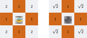
Before we solve our concrete problem, we zoom out a bit to explain the broader framework. In our day-to-day life, we are often looking for distance-minimizing routes. But real-world problems are rarely as neat as walking the straight line from starting point A to end point B. If you’ve ever navigated a city laid out in a grid, like Manhattan or, more locally, Mannheim, you’ll know that walking in a direct straight line from building A to a diagonally opposite building B would often require passing straight through other buildings. Instead, the shortest feasible route involves following two sides of the grid, moving first in one direction and then perpendicular to it, to reach your destination. Here, the underlying geometry, named Taxicab geometry, measures distances by the total path along the streets, not the direct “as the crow flies” Euclidean distance.

For a more complicated example, think of the route a flight takes when crossing continents. Since the Earth is round, it has a smaller circumference the further away from the equator. So the shortest path between Dubai and Los Angeles isn’t the naive straight line crossing the Atlantic Ocean but the arc through the Arctic one.

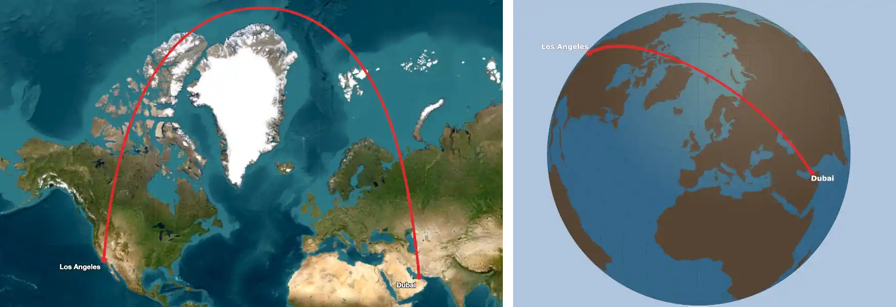
Geometry gives us many well-understood ways of measuring distance, from the familiar straight-line distance to distances along the surface of a sphere. These tools are powerful, but they share one important feature: the shape of the space is known in advance.

In our earlier examples, this was perfectly reasonable. We know that countries lie on a globe, and we know how a city is laid out. New data points do not change that structure – they simply take their place within it. The notion of distance is fixed beforehand.

When working with images, we also place our data points into a space — the feature space introduced above. Each image occupies a well-defined position according to its measured attributes. But here, unlike the globe or the city, the structure of the space is not something we truly understand in advance. We chose the features, and we chose how to measure distances between them. A standard distance, such as the straight-line distance, treats all directions in this space equally. Yet for a given task, some differences between images may matter far more than others.

In such cases, using a single, pre-defined notion of distance may not reflect what we actually care about, for example, whether two images show the same object.

Instead of choosing a distance by hand, we would like the notion of similarity to adapt to the data and to the task at hand. This idea, letting the system learn what “close” should mean, is the central motivation behind metric learning.

Metric Learning: a Machine Learning Framework

Classical mathematical methods for finding good solutions rely on structural assumptions about the problem. They are effective when the landscape of possible solutions has a regular shape, i.e. when small adjustments lead to predictable changes and there is a clear direction in which improvement lies. Problems with this structure are known as convex problems. In such cases, efficient mathematical methods can reliably move toward the best solution.

The space of possible distance functions, however, rarely has this structure. Altering how distance is defined can rearrange the data in complex, and sometimes unexpected, ways. There may be no simple direction that steadily improves the result. In this setting, traditional methods lose much of their power.

Why Convexity Matters

For convex functions on convex domains, every local minimum is also a global minimum. This means there are no misleading valleys, so if we just keep moving in a descent direction, then we reliably move towards an optimal solution (or at least an optimal function value). This property is what makes most classical optimization methods rely on it as a theoretical assumption.

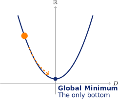
In contrast, the problem of finding an appropriate distance metric is non-convex, producing many local minima and irregular landscapes. As a result, classical optimization methods are insufficient. This is why machine learning approaches, which can explore and adapt to the structure of the data, are used for discovering meaningful metrics.

For Advanced Readers: Convexity in Optimization

You wish to get to know the mathematics? Click here to expand this section!

Optimization problems often take the form
$$
\min_{x \in \mathcal{D}} f(x)
$$

where $f$ is a function and $\mathcal{D}$ is the set of admissible parameters $x$.

Convex Sets

A set $\mathcal{D} \subset \mathbb{R}^n$ is convex if, for any two points in $\mathcal{D}$, the entire line segment between them also lies in $\mathcal{D}$. Formally, for any $x, y \in \mathcal{D}$

$$
\lambda x + (1-\lambda)y \in \mathcal{D}, \quad \forall \lambda \in [0,1].
$$

Geometrically, this means that $\mathcal{D}$ has no holes or inward dents.

Convex Functions

A function $f : \mathcal{D} \to \mathbb{R}$ is convex if the graph of $f$ always lies below the straight line connecting any two of its points. Formally, for all $x, y \in \mathcal{D}$ and all $\lambda \in [0,1]$,

$$
f(\lambda x + (1-\lambda)y) \leq \lambda f(x) + (1-\lambda)f(y).
$$

In one dimension, this corresponds to a u-shaped curve.

Machine learning approaches the problem differently. Rather than specifying a distance formula in advance, it lets data guide the choice. By observing examples of which objects should be regarded as similar and which should not, the system adjusts its internal representation accordingly.

More specifically, metric learning is the branch of machine learning devoted to this task. Its goal is to construct a notion of distance that reflects meaningful relationships in the data. Given examples, it modifies the representation so that related items move closer together and unrelated ones farther apart. To take up our example again, we choose the portrait view of the cottage to be a reference point, and nudge its numerical identification as a collection of pixels closer to the representation of the portrait view than to cows in the field.

The complexity of this task depends on how uniform the data is. Suppose we assume that the same notion of distance works everywhere in the feature space: no matter where we are in the data landscape, distance is measured in exactly the same way. In that case, we are learning what is called a global metric: a single transformation that reshapes the entire feature space uniformly.

In many real-world situations, however, data is not organized so evenly. The structure of the feature space can vary from region to region. Consider the task of judging musical similarity. What it means for two pieces to be “close” may differ entirely depending on whether we are comparing techno tracks or classical compositions. In such cases, relationships between data points depend on context, and a single uniform notion of distance may not suffice.

To handle this, we need something more flexible or local. Riemannian metric learning takes up this task by allowing the notion of distance to change smoothly from point to point. Unlike the Euclidean metric, which measures distance everywhere with the same “straight ruler,” a Riemannian metric tells you how to measure distances on a curved space, like navigating a hilly landscape rather than a perfectly flat map.

Anyone who has looked at a hiking map knows that height information matters. On a flat plane, or a world with no valleys and mountains, i.e. the Euclidean case, the distance between two towns corresponds to the straight line on the map. But in real, uneven terrain, the true distance between two places depends on the ups and downs along the way. Two villages that look close on a flat map may truly be much farther apart if a steep ridge lies between them, because the physically shortest path bends around the terrain instead of following a straight line.

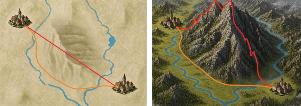
A Riemannian metric works the same way: at every tiny patch of space, it equips you with a “custom-made ruler” that fits exactly to the shape of that patch. This local ruler might be slightly stretched, tilted, or skewed compared to the ruler at another point. But as you move from one point to the next, they change smoothly, so you never experience a sudden jump or jolt in how distances are measured. In this sense, Riemannian metric learning deliberately makes use of “terrain”, the local geometry of the data, to define what similarity means in context, rather than relying on a one-size-fits-all notion of distance.

Once we have a way of measuring distances between things, whether they’re points on a map, images, or even more abstract data, it becomes natural to group similar things together. This is exactly the idea behind one of the simplest and surprisingly powerful tools in machine learning: nearest neighbours algorithms. In classification tasks, for example, we often want to predict the category of a new, unseen data point: here is a new track that came out, is it folk or indie? Let’s check its distance in the space of music. The logic is delightfully human: look at the points nearby, i.e. those most similar according to our chosen metric, and see how they are labelled. If most of your nearest neighbours are classified as “folk”, chances are your new point should be too.

Conclusion

We began with a simple question: why two views of the same cottage can look, to a computer, less alike than a cottage and a field of cows. The answer was not that the computer measured badly, but that it measured with the wrong ruler. A flat, one-size-fits-all distance asks how far apart are these numbers?, when the question we cared about was do these show the same thing? Riemannian metric learning closes that gap by letting the geometry itself be learned: the space bends so that meaningful differences become large and superficial ones become small.

Learning the geometry in this way is not limited to object recognition. Consider comparing two medical scans: small numerical differences may reflect harmless variation, or the early signs of a disease. The way we measure distance between these scans influences what is flagged as significant.

Or think of a music streaming service deciding which song to recommend next. Whether songs are considered “close”, as discussed above, depends on which aspects – rhythm, genre, mood, instrumentation – are emphasized. A learned metric can reshape the notion of similarity to match the user’s listening behaviour.

In each case, the choice of distance is not neutral. By adapting the metric to the task, we do not merely refine a technical detail; we reshape the space in which the problem is posed.

Learning the right geometry can provide a unifying language, one that allows mathematicians and scientists across different disciplines to ask related questions, even when their data and posed problems look very different.