Andreas Floer and the Topology of the Three-Body Problem

Imagine you are trying to predict how three objects move in space – say, the Earth, the Moon, and a spacecraft. You know where they are and how fast they are moving now, but you would like to know how they will behave in a month, a year, or a century.

If there were only two objects, the problem would be easy: their motion would follow simple, predictable orbits (e.g. the Earth’s orbit around the Sun is an ellipse). However, as soon as one adds a third body, all known methods seem to fail – an issue which has stalled scientists for more than three centuries. Perhaps surprisingly, Henri Poincaré showed in the late nineteenth century that the motion of the system was chaotic – not random, but extremely sensitive to initial conditions. This means even tiny changes in position or velocity can lead to wildly different outcomes, making the system almost impossible to forecast in the long term. This problem is what is famously called the Three-Body Problem.

There would be far too many names and milestones to cite to write a full history of the Three-Body Problem. This has already been done countless times (see [3], [4],…), and we shall not pretend to attempt it here. Indeed, the problem has been around since Newton’s Principia Mathematica (1687), and it has not shown many signs of wanting to leave the popular psyché – be it among scientists, in sci-fi, or in pop culture.

The problem has kept inspiring increasingly complicated mathematical theories, just in the hope of gaining a tiny bit more understanding of the equations. In this blog post, I’d like to talk about one mathematician, whose name is rarely cited alongside the words “Three-Body Problem”, yet whose extraordinary insights pushed the boundaries of what was thought possible, and has helped to shape current research.

Andreas Floer was born in 1956 in Duisburg, Germany, and joined the graduate school of UC Berkeley in 1982. His life tragically ended in 1991, but in less than ten years Floer managed to profoundly change how we understand classical physics. He managed a feat which everyone believed impossible: building a bridge between Newton’s equations of motion and a seemingly unrelated field: topology.

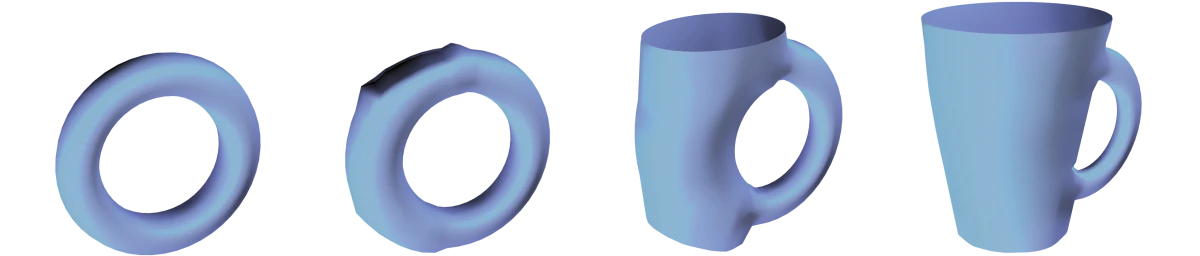
Topology – sometimes called “rubber-sheet geometry” – is the study of shapes, and of those properties which stay the same when stretching, twisting, or bending a shape without tearing it, as if one were moulding play dough. Two shapes are said to be “the same” if one can be continuously deformed into the other in the sense described above. As such, a cup and a doughnut are “the same”, because each can be moulded into the other (the hole of the doughnut becomes the handle of the mug). Likewise, a cube and a sphere are topologically the same. In contrast, a sphere and a doughnut are topologically different: to deform a sphere into a doughnut, one would have to rip a hole into it. Therefore, in essence, topology focuses on the overall shape of objects, forgetting their precise geometry (distances, angles,…)

So what does topology have to do with the Three-Body Problem? How does the connection work? And how come Floer’s name is not world-famous by now? Before we can answer this, we need to talk a little bit about physics.

“The Universe is Lazy”: How Physicists Find Orbits

Let us assume we would like to launch a satellite for Earth observation purposes (water resources monitoring, disaster prevention,…). Such a satellite would have to orbit very close to the surface: between 400 and 600 km, in what we call Low Earth Orbit. As such, we can essentially neglect the influence of other celestial bodies like the Sun or Moon, and only take into account the gravitational pull of the Earth.

To compute the satellite’s orbit, the oldest trick in the book is to use Newton’s three laws of motion, given in his Principia Mathematica. These laws explain how objects move when forces act on them. When combined with the law of universal gravitation, they let us calculate the acceleration the satellite will experience – finding that the acceleration is proportional to the inverse square of the distance, and points in the radial direction towards Earth.

Once we know the satellite’s acceleration, we can work out its trajectory via integration. Loosely speaking, this means we “add up” the tiny changes in motion step by step, allowing us to construct the entire future orbit from a given starting position and initial velocity.

This so-called Two-Body Problem is often given as an exercise to first-year physics students. One can easily show that all of its solutions are conics, that is, they are either:

• Ellipses (corresponding to periodic motion of a satellite, or the Moon, around the Earth) – including the circle as a special case; or:
• Parabolas/hyperbolas (corresponding for instance to the trajectory of an asteroid which flies by the Earth to never return again).

However, there are ways of solving this problem without resorting to Newton’s laws of motion directly. Another popular method comes from something called the Principle of Least Action, which could be summarized by the motto

More precisely, given some trajectory in space, one can define a quantity called the action, which somewhat corresponds to the energetical cost it would take for a physical object to travel along this trajectory.

French polymath Maupertuis discovered in the eighteenth century that the physical trajectories of the object (i.e., the solutions to Newton’s equations of motion) were exactly the ones that minimized the action function. In other words: the universe always tries to minimize the energetical cost of doing anything.

Floer’s Insight

The principle of least action has been around for a long time, and it is now commonly found in every physicist’s toolkit. However, it didn’t spark much interest amongst the pure mathematics community until the 1980s, when Andreas Floer argued that:

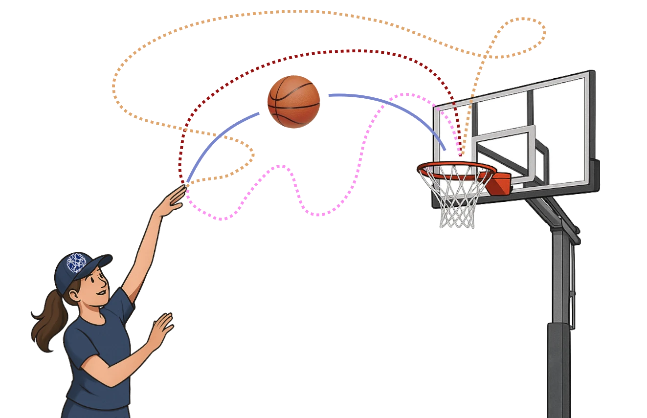
Floer argued that, instead of trying to solve the equations of motion, which might get arbitrarily complicated, we may try and turn this into a problem about shapes. Let us look at a simpler example to illustrate this. Say a basketball player is trying to score a three pointer, and we decide to trace out all trajectories of the ball from their hands into the basket. And by that we really do mean: all trajectories, even ones which may be wildly unrealistic:

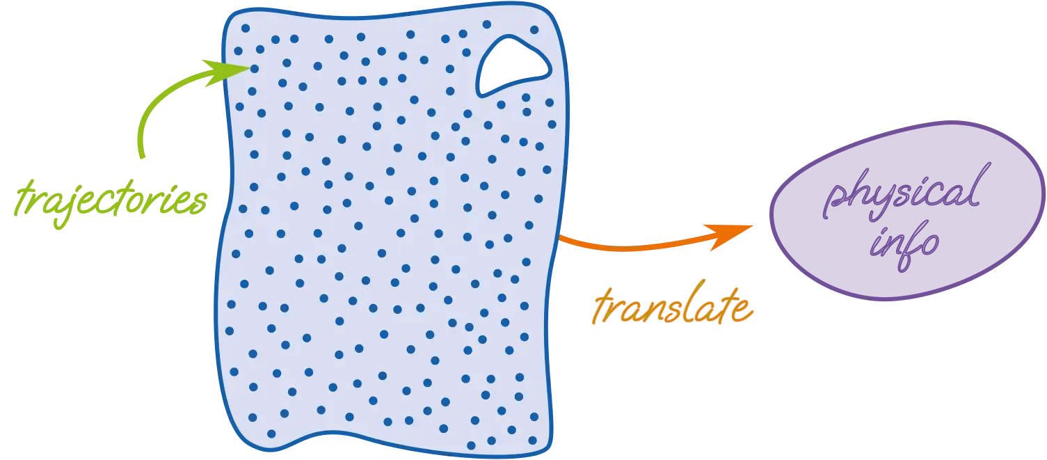
Now, mathematicians introduce a concept, called the “space of trajectories”. This space is an abstract geometric construction: to each trajectory of the basketball (even the unrealistic ones), we assign one point in the space in a prescribed way, keeping track of position and velocity.

The idea of Floer was that to understand the realistic trajectories of the ball, one simply needed to study the shape of this “space of trajectories”. If one understood it well, they could turn that information back into physical terms. In other words, Floer theory acts like a translator.

This space of trajectories is very big (infinite-dimensional, even!) However, mathematicians have methods for probing it. Just like an explorer, before deciding on a route, would try to chart a territory: locating the holes, crevices, rivers, mountains, etc… we too look for interesting features of our space. They tell us which routes are allowed, and which are not. In other words the shape of the “space of trajectories” imposes constraints on the motion.

This explanation, while of course an oversimplification, summarizes the problem-solving strategy quite well. To illustrate it, let us take a recent example from our own research in Heidelberg [2].

An Application: An Interesting Type of Orbits

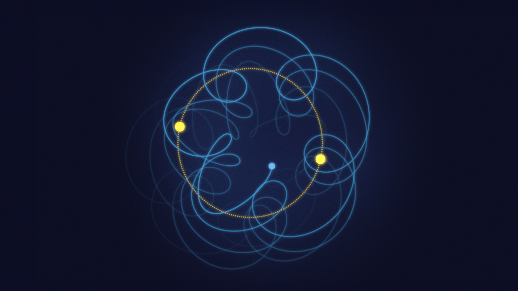
Let us look at a concrete example: imagine a human-made satellite placed near the Earth and Moon, following the classical laws of gravity laid out by Newton.

The motion is already well known for two of the three masses: we know that the Moon and Earth are orbiting in a circle around their common centre of mass (which happens to be inside the Earth). The mass of our satellite is negligible compared to the two large bodies, so we are looking at what astrophysicists call the Circular Restricted variant of the Three-Body Problem.

In this setting, the satellite’s motion is the only unknown – yet, its trajectory is generally complex and chaotic, and therefore highly complicated to predict. While the circular restricted Three-Body Problem imposes restrictive assumptions, it is still of great use for a large number of applications, for instance when trying to send a spacecraft to the Earth-Moon, Jupiter-Europa, Jupiter-Ganymede, or Saturn-Enceladus systems – all of high interest in the space community at the moment.

Let us choose coordinates (x,y,z) such that the x-axis connects the Earth and Moon, and orient the y-axis so that their orbits are confined to the xy-plane.

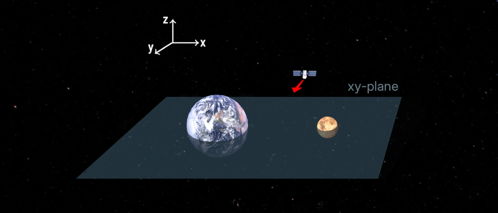
In the above picture, the satellite is drawn normal to the xz-plane. In other words, it belongs to the plane, but its trajectory points orthogonally to it.

Now let us look at a special kind of trajectories. Say you wish to launch a satellite in the above configuration, and pick it up in a similar one at a later time. In other words, the satellite would be normal to the xz-plane at two different points in time (maybe in different locations).

For example, it could be that you own an in-orbit spaceport (a “parking lot for spacecrafts”) stationed in the xz-plane, and would like to launch and capture satellites from it – say if you were asteroid mining, wanting to go out to collect samples and then retrieve them for study.

Then your spacecraft would have to travel along such a trajectory, which we call bi-normal to the xz-plane.

Example: Halo Orbits Around Lagrange Points

A famous example of such trajectories is that of halo orbits. Let us briefly introduce them.

There are five special positions in the Three-Body Problem, where all forces acting on the satellite exactly cancel each other. These “equilibrium locations” are famously known as the Lagrange points. One of them lies in between the Earth and Moon (L1), two on the far side of the Moon and Earth (L2 and L3 respectively), and two form equilateral triangles with the Earth and Moon (L4 and L5). L4 and L5 turn out to be stable, meaning that small disturbances will not cause an object placed there to drift away, but to remain nearby. In the Jupiter-Sun system, L4 and L5 are the locations of Jupiter’s Trojan asteroids – a group of asteroids clustering in these points.

If we wish to keep our satellite close to a Lagrange point, we will need a trajectory that loops around that point. Halo orbits are an example of such trajectories, making them of high interest for space missions. For instance, the James Webb Space Telescope is located in a halo orbit around the Sun-Earth L2 point. Meanwhile, in the Earth-Moon system, the L2 point lies on the far side of the Moon, near the lunar South Pole. The latter has garnered a lot of interest from the space community because of its resources in frozen water and Helium-3, which would allow to set up fuel production, and launching capacity directly on the Moon.

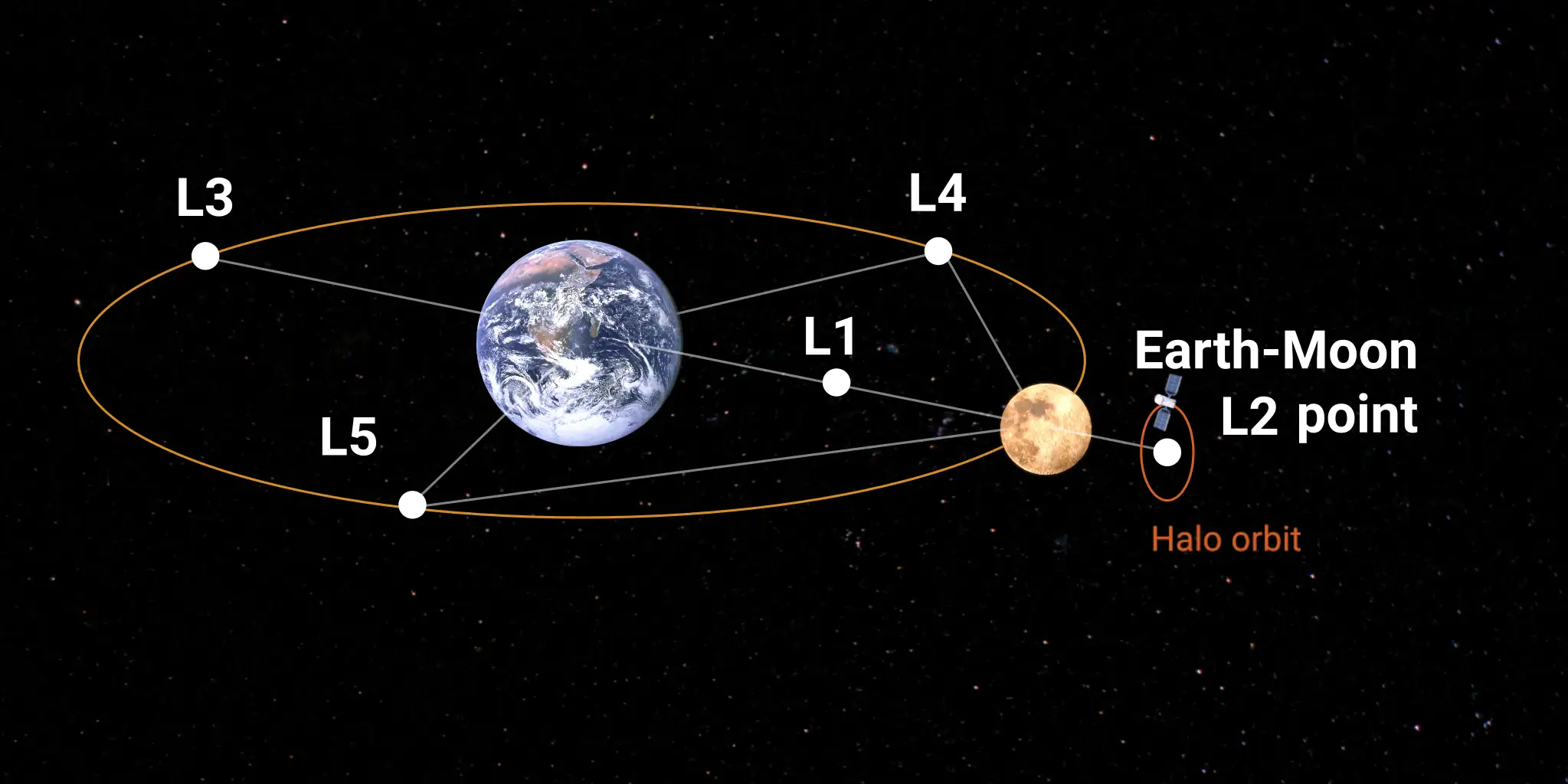
A halo orbit around the Earth-Moon L2 point would allow us to establish constant communication between the Earth and the far-side of the Moon, by placing a relay satellite there. Such communication would be essential for the development of a “Moon base” on the lunar South pole, which is a current project for many members of the current “space club” (the United States, China,…)

In 2018, the China National Space Administration experimented with the satellite Queqiao-1, which travelled on a halo orbit near the Earth-Moon L2 point for seven years.

However, designing such orbits is hard. How do we know which paths are possible and stable? This is where Floer theory enters the picture. As pointed out earlier, Floer theory no longer looks at individual trajectories, but at the space of all trajectories that fit our criteria, and at its shape. In our specific example, the criteria would be:

1. The satellite starts and ends in a specific region (say, near a Lagrange point).
2. It is normal to the xz-plane at two different points in time.
3. It satisfies Newton’s three laws of motion.

In Floer theory, this collection of paths is studied as a mathematical space – a kind of abstract landscape where each point corresponds to a different possible trajectory.

Remarkably, we showed in our research (making one technical assumption, the Weakened Twist Condition) that this space of trajectories was closely related to another, seemingly unrelated space. Imagine you look at the surface of a sphere (e.g. the Earth) and you draw its equator. Now consider a space which would contain all possible paths on this sphere starting and ending in the equator.

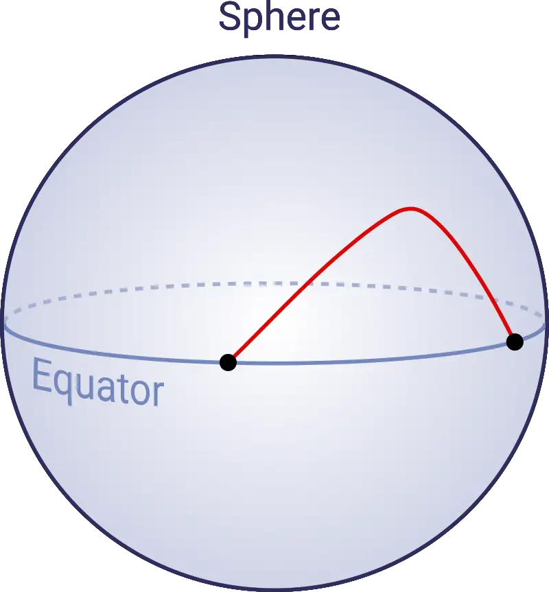
This space of paths is actually quite well-understood, and it is a graduate-level exercise in algebraic topology to show that it has a very rich topology: one can find infinitely many non-equivalent features such as holes, loops, or voids in the space that can’t be “filled in” or shrunk down without making any tears. Mathematicians say that such a space is of infinite-type.

From this, we are able to deduce that our space of trajectories of interest is also of infinite-type. This can be shown to imply that there exist infinitely many trajectories bi-normal to the xz-plane. Thus, we have translated a problem about dynamics and complicated physical motion into a problem about shapes.

While still at a development stage, Floer-theoretical tools are already powerful in astrophysics. If you are an engineer or mission designer trying to find a stable, looping orbit near a Lagrange point (e.g. for a lunar outpost or telescope), it is comforting and strategically useful to know that the dynamical landscape is rich. In particular, it means you are not hunting for a needle in a haystack, but standing in a field full of needles.

This changes computational strategy: rather than brute-force integrating thousands of initial conditions, you can target families of trajectories that you know topologically must be there. Furthermore, this bridge between physics and topology also gives us insights into how our trajectories may behave if one slightly perturbs the initial data (the mass of the bodies, the energy,…), providing concrete applications to mission design.

Example: Voyager Trajectory

Now that we have played this game once, we can do it with other types of trajectories. Such techniques had originally been experimented with for periodic orbits (Moreno, van Koert 2021), and then for collision trajectories (Moreno, Limoge 2024). From an engineering point-of-view, collision trajectories are quite interesting. First of all, knowing where they are sounds important for avoiding them. More interestingly, if our satellite is on a collision trajectory, and we slightly perturb it (say by using thrusters), we will obtain a trajectory of close fly-by, which can then be used for gravitational assist (see for example the Voyager I and II probes, which used the gas giants’ gravitational pull to propel themselves into space, far beyond the confines of our solar system).

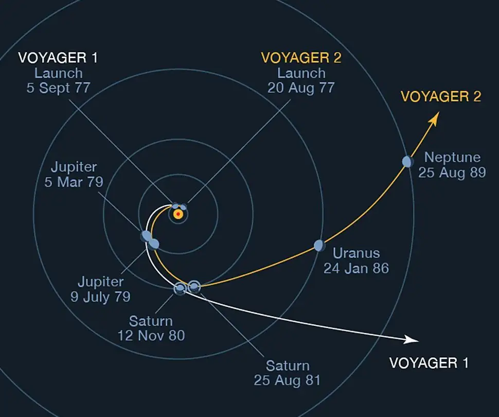
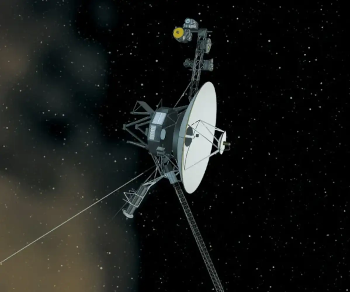
At the time of writing this article, Voyager I and II are at respective distances of 24.9 billion and 20.8 billion kilometres from the Earth.

So Why Is the Three-Body Problem So Hard?

The overall strategy behind Floer theory is roughly always the same:

• Start from a hard physics problem (e.g. studying a specific type of orbits);
• Reduce to an “easy” topology problem (e.g. understanding paths on the sphere).

It may seem almost magical at first. The reason Floer’s name has remained niche, and struggled to make it outside of the geometric community is because despite being revolutionary, his theory is incredibly difficult to construct. You might see experts in the field boasting of their proofs being only a few hundred pages long, or firmly believing in results, which by every metric seem true and agreed upon by the community, but may never be proved because of the sheer amount of technical work required.

In a way, using Floer theory to do physics might feel like using a wrecking ball to hammer down a nail. Floer’s intuition is marvellous, but to bring it to fruition one needs to go through years of rigorous functional analysis, abstract algebra, and differential geometry. Still, it is incredibly useful for those cases where you don’t have a hammer. And while applications to astrophysics are still very new, the insight they give us into using topology for understanding orbits fundamentally changes how we look at the Three-Body Problem.

Overall, the Three-Body Problem has inspired the birth of many new mathematical theories, and survived them all. For instance, Poincaré essentially pioneered the fields of dynamical systems and topology for the very purpose of understanding the Three-Body Problem. His swan song, published a few months before his death, and now referred to as “Poincaré’s last geometric theorem”, sketched a strategy for finding trajectories – a strategy still used to this day (e.g. [2]) which has influenced the whole field of dynamical systems, far beyond the problem it was intended for.

Likely, the Three-Body Problem will keep forcing the creation of new mathematical theories, and survive many more, for quite some time. It may end up as one of the most humbling problems in our community, for unlike other famous questions (the Riemann hypothesis, the Hodge conjecture, the Navier-Stokes equations,…), this one is deceptively simple to state. Almost too simple: we want to understand the motion of three objects in space. Yet no matter how elaborate our models become, the answer keeps eluding us, and it seems we have to content ourselves with slowly chipping away at the surface of the problem, decades at a time.

“There’s this emperor, and he asks this shepherd’s boy ‘How many seconds in eternity?’ And the shepherd’s boy says, ‘There’s this mountain of pure diamond. It takes an hour to climb it and an hour to go around it, and every hundred years a little bird comes and sharpens its beak on the diamond mountain. When the entire mountain is chiselled away, the first second of eternity will have passed.’ You may think that’s a hell of a long time. Personally, I think that’s a hell of a bird.”

–Peter Capaldi, Doctor Who: “Heaven Sent”, written by Steven Moffat, BBC, 2015.

Based on a fairy tale by the Brothers Grimm.

References